This page was generated from notebooks/0C-LogRatioEstimator_Ndim.ipynb.

LogRatioEstimator_Ndim¶

First we need some imports.

[1]:

%load_ext autoreload
%autoreload 2

[2]:

import numpy as np
from scipy import stats
import pylab as plt
import torch
import swyft

Training data¶

Now we generate training data. As simple example, we consider the model

\[x = z + \epsilon\]

where the parameter \(z \sim \mathcal{N}(\mu = 0, \sigma = 1)\) is standard normal distributed, and \(\epsilon \sim \mathcal{N}(\mu = 0, \sigma = 0.1)\) is a small noise contribution. We are interested in the posterior of \(z\) given a measurement of parameter \(x\).

[3]:

N = 100000  # Number of samples
z = np.random.rand(N, 3)*2 - 1
r = (z[:,0]**2 + z[:,1]**2)**0.5
x = r.reshape(N, 1) + np.random.randn(N, 1)*0.1

Training data that is kept in memory is stored in a swyft.Samples object.

[4]:

samples = swyft.Samples(x = x, z = z)

Inference network¶

The inference network is an instance of swyft.SwyftModule. It estimates ratios of the form

\[r(A; B) = \frac{p(A, B)}{p(A)p(B)}\;,\]

where \(A\) and \(B\) refer to any subset of variables in the training data. In the below example, we set \(A \to x\) and \(B \to z\).

We use here a standard dense network, swyft.RatioEstimatorMLP1d, for mapping \(x\) and \(z\) onto a ratio estimator object.

[5]:

class Network(swyft.SwyftModule):
    def __init__(self):
        super().__init__()
        marginals = ((0, 1),)
        self.logratios1 = swyft.LogRatioEstimator_1dim(num_features = 1, num_params = 3, varnames = 'z')
        self.logratios2 = swyft.LogRatioEstimator_Ndim(num_features = 1, marginals = marginals, varnames = 'z')

    def forward(self, A, B):
        logratios1 = self.logratios1(A['x'], B['z'])
        logratios2 = self.logratios2(A['x'], B['z'])
        return logratios1, logratios2

Trainer¶

Training is now done using the SwyftTrainer class, which extends pytorch_lightning.Trainer by methods like infer (see below).

[6]:

trainer = swyft.SwyftTrainer(accelerator = 'gpu', devices=1, max_epochs = 3, precision = 64)

GPU available: True (cuda), used: True
TPU available: False, using: 0 TPU cores
IPU available: False, using: 0 IPUs
HPU available: False, using: 0 HPUs

The swyft.Samples class provides convenience functions to generate data loaders for training and validation data.

[7]:

dm = swyft.SwyftDataModule(samples, fractions = [0.8, 0.02, 0.1], num_workers = 3, batch_size = 256)

[8]:

network = Network()

[9]:

trainer.fit(network, dm)

/home/weniger/miniconda3b/envs/zero/lib/python3.9/site-packages/pytorch_lightning/callbacks/model_checkpoint.py:616: UserWarning: Checkpoint directory /home/weniger/codes/swyft/notebooks/lightning_logs/version_10034687/checkpoints exists and is not empty.
  rank_zero_warn(f"Checkpoint directory {dirpath} exists and is not empty.")
LOCAL_RANK: 0 - CUDA_VISIBLE_DEVICES: [0]

  | Name       | Type                   | Params
------------------------------------------------------
0 | logratios1 | LogRatioEstimator_1dim | 52.2 K
1 | logratios2 | LogRatioEstimator_Ndim | 17.5 K
------------------------------------------------------
69.7 K    Trainable params
0         Non-trainable params
69.7 K    Total params
0.558     Total estimated model params size (MB)

Epoch 0:  97%|█████████▋| 340/349 [00:05<00:00, 64.09it/s, loss=-0.846, v_num=1e+7]
Validation: 0it [00:00, ?it/s]
Validation:   0%|          | 0/9 [00:00<?, ?it/s]
Validation DataLoader 0:   0%|          | 0/9 [00:00<?, ?it/s]
Epoch 0:  98%|█████████▊| 341/349 [00:05<00:00, 59.77it/s, loss=-0.846, v_num=1e+7]
Epoch 0:  98%|█████████▊| 342/349 [00:05<00:00, 59.82it/s, loss=-0.846, v_num=1e+7]
Epoch 0:  98%|█████████▊| 343/349 [00:05<00:00, 59.87it/s, loss=-0.846, v_num=1e+7]
Epoch 0:  99%|█████████▊| 344/349 [00:05<00:00, 59.92it/s, loss=-0.846, v_num=1e+7]
Epoch 0:  99%|█████████▉| 345/349 [00:05<00:00, 60.01it/s, loss=-0.846, v_num=1e+7]
Epoch 0:  99%|█████████▉| 346/349 [00:05<00:00, 60.09it/s, loss=-0.846, v_num=1e+7]
Epoch 0:  99%|█████████▉| 347/349 [00:05<00:00, 60.20it/s, loss=-0.846, v_num=1e+7]
Epoch 0: 100%|█████████▉| 348/349 [00:05<00:00, 60.30it/s, loss=-0.846, v_num=1e+7]
Epoch 0: 100%|██████████| 349/349 [00:05<00:00, 60.38it/s, loss=-0.846, v_num=1e+7, val_loss=-.902]
Epoch 1:  97%|█████████▋| 340/349 [00:05<00:00, 64.40it/s, loss=-0.873, v_num=1e+7, val_loss=-.902]
Validation: 0it [00:00, ?it/s]
Validation:   0%|          | 0/9 [00:00<?, ?it/s]
Validation DataLoader 0:   0%|          | 0/9 [00:00<?, ?it/s]
Epoch 1:  98%|█████████▊| 341/349 [00:05<00:00, 60.30it/s, loss=-0.873, v_num=1e+7, val_loss=-.902]
Epoch 1:  98%|█████████▊| 342/349 [00:05<00:00, 60.41it/s, loss=-0.873, v_num=1e+7, val_loss=-.902]
Epoch 1:  98%|█████████▊| 343/349 [00:05<00:00, 60.50it/s, loss=-0.873, v_num=1e+7, val_loss=-.902]
Epoch 1:  99%|█████████▊| 344/349 [00:05<00:00, 60.61it/s, loss=-0.873, v_num=1e+7, val_loss=-.902]
Epoch 1:  99%|█████████▉| 345/349 [00:05<00:00, 60.73it/s, loss=-0.873, v_num=1e+7, val_loss=-.902]
Epoch 1:  99%|█████████▉| 346/349 [00:05<00:00, 60.83it/s, loss=-0.873, v_num=1e+7, val_loss=-.902]
Epoch 1:  99%|█████████▉| 347/349 [00:05<00:00, 60.94it/s, loss=-0.873, v_num=1e+7, val_loss=-.902]
Epoch 1: 100%|█████████▉| 348/349 [00:05<00:00, 61.04it/s, loss=-0.873, v_num=1e+7, val_loss=-.902]
Epoch 1: 100%|██████████| 349/349 [00:05<00:00, 61.11it/s, loss=-0.873, v_num=1e+7, val_loss=-.906]
Epoch 2:  97%|█████████▋| 340/349 [00:05<00:00, 64.88it/s, loss=-0.874, v_num=1e+7, val_loss=-.906]
Validation: 0it [00:00, ?it/s]
Validation:   0%|          | 0/9 [00:00<?, ?it/s]
Validation DataLoader 0:   0%|          | 0/9 [00:00<?, ?it/s]
Epoch 2:  98%|█████████▊| 341/349 [00:05<00:00, 62.41it/s, loss=-0.874, v_num=1e+7, val_loss=-.906]
Epoch 2:  98%|█████████▊| 342/349 [00:05<00:00, 61.11it/s, loss=-0.874, v_num=1e+7, val_loss=-.906]
Epoch 2:  98%|█████████▊| 343/349 [00:05<00:00, 61.20it/s, loss=-0.874, v_num=1e+7, val_loss=-.906]
Epoch 2:  99%|█████████▊| 344/349 [00:05<00:00, 61.31it/s, loss=-0.874, v_num=1e+7, val_loss=-.906]
Epoch 2:  99%|█████████▉| 345/349 [00:05<00:00, 61.43it/s, loss=-0.874, v_num=1e+7, val_loss=-.906]
Epoch 2:  99%|█████████▉| 346/349 [00:05<00:00, 61.53it/s, loss=-0.874, v_num=1e+7, val_loss=-.906]
Epoch 2:  99%|█████████▉| 347/349 [00:05<00:00, 61.64it/s, loss=-0.874, v_num=1e+7, val_loss=-.906]
Epoch 2: 100%|█████████▉| 348/349 [00:05<00:00, 61.74it/s, loss=-0.874, v_num=1e+7, val_loss=-.906]
Epoch 2: 100%|██████████| 349/349 [00:05<00:00, 61.80it/s, loss=-0.874, v_num=1e+7, val_loss=-.869]
Epoch 2: 100%|██████████| 349/349 [00:05<00:00, 61.77it/s, loss=-0.874, v_num=1e+7, val_loss=-.869]

`Trainer.fit` stopped: `max_epochs=3` reached.

Epoch 2: 100%|██████████| 349/349 [00:05<00:00, 61.38it/s, loss=-0.874, v_num=1e+7, val_loss=-.869]

Inference¶

We assume that we measure the values \(x=0.2\).

[10]:

x0 = 0.5

We first generate a large number of prior samples.

[11]:

B = swyft.Samples(z = np.random.rand(1000000, 3)*2-1)

Swyft provides the method infer in order to efficiently evaluate the inference network. That method takes either dataloaders or individual samples (i.e. dictionaries of tensors) as input. This efficiently evaluates the ratio \(r(x; z)\) for a large number of prior samples \(z\) for a fixed values of \(x\).

[12]:

A = swyft.Sample(x = np.array([x0]))

[13]:

predictions = trainer.infer(network, A, B)

LOCAL_RANK: 0 - CUDA_VISIBLE_DEVICES: [0]

Predicting DataLoader 0:   2%|▏         | 17/977 [00:00<00:09, 96.02it/s]

/home/weniger/miniconda3b/envs/zero/lib/python3.9/site-packages/pytorch_lightning/loops/epoch/prediction_epoch_loop.py:173: UserWarning: Lightning couldn't infer the indices fetched for your dataloader.
  warning_cache.warn("Lightning couldn't infer the indices fetched for your dataloader.")

Predicting DataLoader 0: 100%|██████████| 977/977 [00:10<00:00, 90.64it/s]

Plot results¶

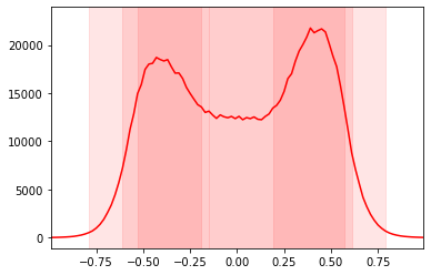
First we obtain samples from the posterior, using subsampling with a weight that happens to be given by \(e^r\).

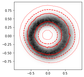
[14]:

swyft.plot_2d(predictions, "z[0]", "z[1]", bins = 100, smooth = 0.5, color = 'r', ax = plt.gca(), cmap = 'gray_r');

../_images/notebooks_0C-LogRatioEstimator_Ndim_24_0.png

[15]:

swyft.plot_1d(predictions, "z[0]", bins = 100, smooth = 0, color = 'r', ax = plt.gca());

../_images/notebooks_0C-LogRatioEstimator_Ndim_25_0.png

[16]:

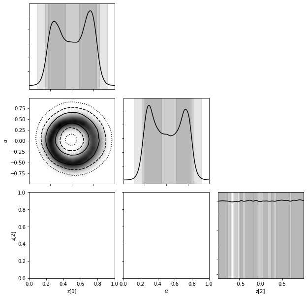
labeler = {'z[1]': r"$\alpha$"}
swyft.corner(predictions, ('z[0]', 'z[1]', 'z[2]'), labeler = labeler, bins = 200, smooth = 3);

../_images/notebooks_0C-LogRatioEstimator_Ndim_26_0.png

[ ]:

This page was generated from notebooks/0C-LogRatioEstimator_Ndim.ipynb.