This page was generated from notebooks/1A - Image analysis and rings.ipynb.

Example A - Rings

(works only with Swyft 0.4.4; to be updated soon)

Authors: Noemi Anau Montel, James Alvey, Christoph Weniger

Last update: 2 August 2023

Purpose: In this example we will use a gravitational lensing toy simulator. By reducing training data variance with truncation rounds, we will see our network converge to tighter posteriors.

Code

%load_ext tensorboard
import tensorflow as tf
import datetime, os

import numpy as np
import swyft
import pylab as plt
from scipy import stats
import torch
from pytorch_lightning.callbacks import LearningRateMonitor, ModelCheckpoint
from pytorch_lightning.callbacks.early_stopping import EarlyStopping
from pytorch_lightning import loggers as pl_loggers

Let’s start by considering a toy model for producing simulated images of graviationally lensed systems. The radius r would then correspond to the “Einstein radius” of the gravitational lensing system and tell us something about the mass of the lensing galaxy. The width w would correspond to the size of the lensed source galaxy. We will also add random distortions in terms of lines to test just how difficult we can make the problem while still learning the parameters.

Here is our simulator:

class Simulator(swyft.Simulator):
    def __init__(self, bounds=None):
        super().__init__()
        self.transform_samples = swyft.to_numpy32
        x = np.linspace(-2, 2, 32)
        self.X, self.Y = np.meshgrid(x, x)
        self.bounds = bounds

    def z(self):
        return swyft.RectBoundSampler(stats.uniform(np.array([0.1, 0.01]), np.array([1, 0.3])), bounds = self.bounds)()

    def mu(self, z):
        r, w = z
        # Random position of the ring
        x0, y0 = np.random.uniform(-1, 1, 2)
        R = ((self.X-x0)**2 + (self.Y-y0)**2)**0.5
        mu = np.exp(-(R-r)**2/w**2/2)

        # Add random distortions in terms of lines
        for _ in range(20):
            xr = np.random.rand(2)
            mu += 0.8*np.exp(-(self.X*xr[0]+self.Y*(1-xr[0])-xr[1])**2/0.01**2)

        # Standard variance and zero mean
        mu -= mu.mean()
        mu /= mu.std()
        return mu

    def img(self, mu):
        # Add image noise
        return mu + np.random.randn(*mu.shape)*0.3

    def build(self, graph):
        z = graph.node('z', self.z)
        mu = graph.node('mu', self.mu, z)
        img = graph.node('img', self.img, mu)

sim = Simulator()
samples = sim.sample(10000)

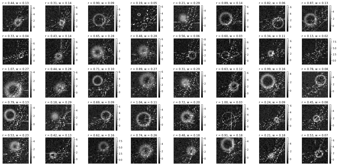
Let’s visualize our data

fig = plt.figure(figsize=(20, 10))
for i in range(40):
  plt.subplot(5,8,i+1); plt.tight_layout()
  plt.imshow(samples['img'][i], cmap='gray', interpolation='none')
  plt.title("r = {:.2f}".format(samples['z'][i][0].item()) + ", w = {:.2f}".format(samples['z'][i][1].item()))
  plt.xticks([]); plt.yticks([]); plt.colorbar()

We will now try to estimate the radius and width of the ring. We start by considering a simple Linear layer as an embedding network.

class Network(swyft.SwyftModule):
    def __init__(self, lr = 1e-3, gamma = 1.):
        super().__init__()

        # We define a custom optimizer with learning rate decay
        self.optimizer_init = swyft.OptimizerInit(torch.optim.Adam, dict(lr = lr),
              torch.optim.lr_scheduler.ReduceLROnPlateau, dict(factor = 0.3, patience=5))

        self.logratios1 = swyft.LogRatioEstimator_1dim(num_features = 16, num_params = 2, varnames = 'z', dropout = 0.0)
        self.logratios2 = swyft.LogRatioEstimator_Ndim(num_features = 16, marginals = ((0,1),), varnames = 'z', dropout = 0.0)
        self.net = torch.nn.Sequential(
          torch.nn.Flatten(),
          torch.nn.Linear(32*32, 16),
        )

    def forward(self, A, B):
        f = self.net(A['img'].unsqueeze(1)).squeeze(1)
        logratios1 = self.logratios1(f, B['z'])
        logratios2 = self.logratios2(f, B['z'])
        return logratios1, logratios2

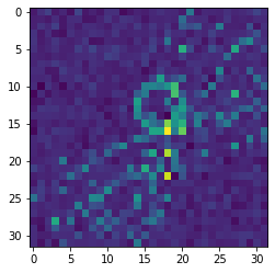
Let’s define our random target observations.

obs = swyft.Sample(sim.sample())
plt.imshow(obs['img'])
print("z =", obs['z'])

z = [0.3825986  0.05225621]

Inference is run as usual, here with some extra code for monitoring the learning rate, early stopping.

dm = swyft.SwyftDataModule(samples, fractions = [0.7, 0.2, 0.1], batch_size = 32)

lr_monitor = LearningRateMonitor(logging_interval='step')
early_stopping_callback = EarlyStopping(monitor='val_loss', min_delta = 0., patience=3, verbose=False, mode='min')
checkpoint_callback = ModelCheckpoint(monitor='val_loss', dirpath='./logs/', filename='rings_{epoch}_{val_loss:.2f}_{train_loss:.2f}', mode='min')
logger = pl_loggers.TensorBoardLogger(save_dir='./logs/', name='rings_logs', version=None)

trainer = swyft.SwyftTrainer(accelerator = 'gpu', max_epochs = 20, logger=logger, callbacks=[lr_monitor, early_stopping_callback, checkpoint_callback],)
network = Network()
trainer.fit(network, dm)

INFO:pytorch_lightning.utilities.rank_zero:GPU available: True (cuda), used: True
INFO:pytorch_lightning.utilities.rank_zero:TPU available: False, using: 0 TPU cores
INFO:pytorch_lightning.utilities.rank_zero:IPU available: False, using: 0 IPUs
INFO:pytorch_lightning.utilities.rank_zero:HPU available: False, using: 0 HPUs
WARNING:pytorch_lightning.loggers.tensorboard:Missing logger folder: ./logs/rings_logs
INFO:pytorch_lightning.accelerators.cuda:LOCAL_RANK: 0 - CUDA_VISIBLE_DEVICES: [0]
INFO:pytorch_lightning.callbacks.model_summary:
  | Name       | Type                   | Params
------------------------------------------------------
0 | logratios1 | LogRatioEstimator_1dim | 36.7 K
1 | logratios2 | LogRatioEstimator_Ndim | 18.4 K
2 | net        | Sequential             | 16.4 K
------------------------------------------------------
71.6 K    Trainable params
0         Non-trainable params
71.6 K    Total params
0.286     Total estimated model params size (MB)

We can evaluate the loss function on the test training dataset.

checkpoint_callback.to_yaml("./logs/rings.yaml")
ckpt_path = swyft.best_from_yaml("./logs/rings.yaml")
trainer.test(network, dm, ckpt_path = ckpt_path)

INFO:pytorch_lightning.utilities.rank_zero:Restoring states from the checkpoint path at /content/logs/rings_epoch=2_val_loss=-1.33_train_loss=-1.38.ckpt
INFO:pytorch_lightning.accelerators.cuda:LOCAL_RANK: 0 - CUDA_VISIBLE_DEVICES: [0]
INFO:pytorch_lightning.utilities.rank_zero:Loaded model weights from checkpoint at /content/logs/rings_epoch=2_val_loss=-1.33_train_loss=-1.38.ckpt

────────────────────────────────────────────────────────────────────────────────────────────────────────────────────────
       Test metric             DataLoader 0
────────────────────────────────────────────────────────────────────────────────────────────────────────────────────────
        test_loss           -1.3773839473724365
────────────────────────────────────────────────────────────────────────────────────────────────────────────────────────

[{'test_loss': -1.3773839473724365}]

%tensorboard --logdir ./logs/rings_logs/

Let’s infer our predictions as usual…

prior_samples = sim.sample(N = 10000, targets = ['z'])
predictions = trainer.infer(network, obs, prior_samples)

INFO:pytorch_lightning.accelerators.cuda:LOCAL_RANK: 0 - CUDA_VISIBLE_DEVICES: [0]

/usr/local/lib/python3.8/dist-packages/pytorch_lightning/loops/epoch/prediction_epoch_loop.py:173: UserWarning: Lightning couldn't infer the indices fetched for your dataloader.
  warning_cache.warn("Lightning couldn't infer the indices fetched for your dataloader.")

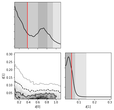
… and plot them

truth = {k: v for k, v in zip(["z[%i]"%i for i in range(2)], obs['z'])}
swyft.plot_corner(predictions, ('z[0]', 'z[1]'), bins = 200, smooth = 3, truth=truth);

Exercise

With a simple linear layer we are starting to learn something, but we can do better.

1. Add noise resampling.

# You solution

dm = swyft.SwyftDataModule(samples, fractions = [0.7, 0.2, 0.1], batch_size = 32, on_after_load_sample=sim.get_resampler(targets = ["img"]))

2. Improving the embedding network by adding additional convolutional, max pooling, and non-linear activation function layers. We can also try changing the dropout in the ratio estimator. You can copy&paste with from the MNIST example (with appropriate addoptions).

# Your solution

3. Add a truncation rounds to zoom into the relevant parameter space.

# Your solution

This page was generated from notebooks/1A - Image analysis and rings.ipynb.