This page was generated from notebooks/0I - Model comparison.ipynb.
I - Model comparison#
Authors: Noemi Anau Montel, James Alvey, Christoph Weniger
Last update: 27 April 2023
Proposal: How to perform model comparison in swyft estimating the Bayes factor.
Key take-away messages: Learn how to use the switch method to introduce conditional dependency in the computational graph.
Code#
[ ]:
import numpy as np
from scipy import stats
import pylab as plt
import torch
import swyft
Although we cannot direclty estimate the evidence of data, \(p(\mathbf x)\), given a model, we can use neural ratio estimation to estimate the ratio of two marginal likelihoods, also known as the Bayes factor.
If we have to models \(M0\) and \(M1\), we can estimate the Bayes factor
by taking the ratio of the ratios
and
The evidence \(p(\mathbf x)\) would cancel out in this case.
As an example, let us consider two simulators. We then define a composite simulator which has as its only parameter a discrete value that decides which of the base simulators to use. This exploits the fact that simulators can be nested in Swyft.
[ ]:
class Sim_M0(swyft.Simulator):
    def __init__(self):
        super().__init__()
        self.transform_samples = swyft.to_numpy32

    def build(self, graph):
        x = graph.node('x', lambda: np.random.randn(10))

class Sim_M1(swyft.Simulator):
    def __init__(self):
        super().__init__()
        self.transform_samples = swyft.to_numpy32

    def build(self, graph):
        x = graph.node('x', lambda: np.random.randn(10)*2.1)

class Simulator(swyft.Simulator):
    def __init__(self):
        super().__init__()
        self.transform_samples = swyft.to_numpy32
        self.sim0 = Sim_M0()
        self.sim1 = Sim_M1()

    def build(self, graph):
        d = graph.node('d', lambda: np.random.choice(2, size=1).astype(float))
        with graph.prefix("M0/"):
            self.sim0.build(graph)
        with graph.prefix("M1/"):
            self.sim1.build(graph)
        x = graph.switch('x', [graph["M0/x"], graph["M1/x"]], d)

sim = Simulator()
Note: - We use here the switch method, which introduces some conditional dependencies in the computational graph. Depending on the value of d, x is assigned different values. The switch statements make sure that parameter dependencies are properly propagated and only relevant computational nodes are executed. - We combine the graphs from multiple models by explicitly calling the build method of sub-models. - We use the prefix method to prepend some additional string to
the parameter names of the included sub-models. This acts as neat namespace.
Finally, we can start with generating samples.
[ ]:
samples = sim.sample(10000)
Inference network and training work similar to before. (Note that for more than 2 classes, it would be a good idea to use one-hot encoding before passing parameters to the LogRatioEstimator - we do not worry about this here).
[ ]:
class Network(swyft.SwyftModule):
    def __init__(self):
        super().__init__()
        self.logratios = swyft.LogRatioEstimator_1dim(num_features = 10, num_params = 1, varnames = 'd')

    def forward(self, A, B):
        logratios = self.logratios(A['x'], B['d'])
        return logratios

trainer = swyft.SwyftTrainer(accelerator = 'gpu', devices=1, max_epochs = 10, precision = 64)
dm = swyft.SwyftDataModule(samples, fractions = [0.7, 0.3, 0.1], num_workers = 0, batch_size = 64)
network = Network()
trainer.fit(network, dm)
INFO:pytorch_lightning.utilities.rank_zero:GPU available: True (cuda), used: True
INFO:pytorch_lightning.utilities.rank_zero:TPU available: False, using: 0 TPU cores
INFO:pytorch_lightning.utilities.rank_zero:IPU available: False, using: 0 IPUs
INFO:pytorch_lightning.utilities.rank_zero:HPU available: False, using: 0 HPUs
INFO:pytorch_lightning.accelerators.cuda:LOCAL_RANK: 0 - CUDA_VISIBLE_DEVICES: [0]
INFO:pytorch_lightning.callbacks.model_summary:
  | Name      | Type                   | Params
-----------------------------------------------------
0 | logratios | LogRatioEstimator_1dim | 18.0 K
-----------------------------------------------------
18.0 K    Trainable params
0         Non-trainable params
18.0 K    Total params
0.144     Total estimated model params size (MB)
INFO:pytorch_lightning.utilities.rank_zero:`Trainer.fit` stopped: `max_epochs=10` reached.
Finally, we can perform classification. As usual, we sample from the prior and infer. Then we can use the get_class_probs function to turn predictions into class probabilities.
[ ]:
obs = sim.sample()
prior_samples = sim.sample(2_000, targets = ['d'])
predictions = trainer.infer(network, obs, prior_samples)
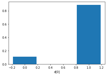
probs = swyft.get_class_probs(predictions, 'd[0]')
plt.bar([0, 1], probs, width = 0.37, log = False)
plt.xlabel("d[0]");
K = probs[1]/probs[0]
print("True class =", obs['d'][0])
print("Bayes factor K = p(d=1|x)/p(d=0|x) =", K)
INFO:pytorch_lightning.accelerators.cuda:LOCAL_RANK: 0 - CUDA_VISIBLE_DEVICES: [0]
True class = 1.0
Bayes factor K = p(d=1|x)/p(d=0|x) = 8.032159126404032
Exercises#
Add an additional class into the simulator above to try and distinguish between three models - what are the relevant Bayes factors in this case?
[ ]:
# Code goes here
This page was generated from notebooks/0I - Model comparison.ipynb.