This page was generated from notebooks/0A - SwyftModule.ipynb.

A - Building inference networks with SwyftModule

Authors: Noemi Anau Montel, James Alvey, Christoph Weniger

Last update: 27 April 2023

Purpose: We go through the basic steps of performing parameter inference with Swyft.

Note: As is always the case when dealing with training of artificial neural networks, obtaining optimal results depends on a proper setting of training and network parameters. This will be discussed later.

Key take-away messages: Understand swyft’s main functions for data and dataloaders (swyft.Samples, swyft.SwyftDataModule), networks (swyft.SwyftModule) and training/inference (swyft.SwyftTrainer).

Code

Setup

First we need some imports.

import numpy as np
import pylab as plt
import swyft

Training data

Now we generate training data. As a simple example, we consider the model

\[x = z + \epsilon\]

where the parameter \(z \sim \mathcal{U}(-1, 1)\) is drawn from the uniform distribution, and \(\epsilon \sim \mathcal{N}(\mu = 0, \sigma = 0.1)\) is small additive noise. We are interested in the posterior of \(z\) given a measurement of parameter \(x\).

Let us generate some samples first, here by using basic numpy functionality.

N = 3000  # Number of samples
z = np.random.rand(N, 1)*2-1  # Uniform prior over [-1, 1]
x = z + np.random.randn(N, 1)*0.2

Note that the shape of the z and x arrays is (n_samples, 1). The first dimension corresponds to the number of samples. Subsequent dimensions correspond to data and parameter shapes (here simply one in both cases).

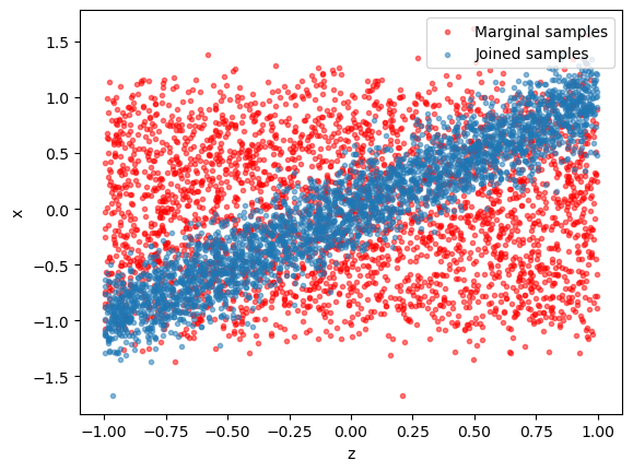
It is instructive to visualize the training data. - Blue dots: generated \((x, z)\) pairs (“jointly sampled”) - Red dots: scrambled \((x, z)\) pairs (“marginally sampled”).

plt.scatter(z[:,0], np.random.permutation(x[:,0]), alpha = 0.5, marker='.', color='r', label = "Marginal samples"); plt.xlabel("z"); plt.ylabel("x");
plt.scatter(z[:,0], x[:,0], alpha = 0.5, marker='.', label = "Joined samples"); plt.xlabel("z"); plt.ylabel("x"); plt.legend(loc = 1)

<matplotlib.legend.Legend at 0x7f00f737c700>

Training data that is kept in memory is stored in a swyft.Samples object.

samples = swyft.Samples(x = x, z = z)

Inference network

The inference network is an instance of swyft.SwyftModule. It estimates ratios of the form

\[r(a; b) = \frac{p(a, b)}{p(a)p(b)}\;,\]

where \(a\) and \(b\) refer to any components of the training data. In the below example, we set \(a \to x\) and \(b \to z\).

class Network(swyft.SwyftModule):
    def __init__(self):
        super().__init__()
        self.logratios = swyft.LogRatioEstimator_1dim(num_features = 1, num_params = 1, varnames = 'z')

    def forward(self, A, B):
        return self.logratios(A['x'], B['z'])

Swyft comes with a few default networks. Here we use swyft.LogRatioEstimator_1dim, which is a dense network that estimates (potentially multiple) one-dimensional posteriors. In the present example, the length of the parameter vector (num_params) and data vectors (num_features) are one.

Training

Training is now done using the SwyftTrainer class, which extends pytorch_lightning.Trainer by methods like infer (see below). Since our training data is double precision in this example, we have to set precision = 64.

trainer = swyft.SwyftTrainer(accelerator = 'gpu', devices = 1, max_epochs = 3, precision = 64)

/home/weniger/.conda/envs/lensing/lib/python3.9/site-packages/lightning_fabric/plugins/environments/slurm.py:166: PossibleUserWarning: The `srun` command is available on your system but is not used. HINT: If your intention is to run Lightning on SLURM, prepend your python command with `srun` like so: srun python /home/weniger/.conda/envs/lensing/lib/python3.9/site ...
  rank_zero_warn(
GPU available: True (cuda), used: True
TPU available: False, using: 0 TPU cores
IPU available: False, using: 0 IPUs
HPU available: False, using: 0 HPUs

The swyft.SwyftDataModule class provides convenience functions to generate data loaders for training and validation data. We preserve 20% of samples for validation.

dm = swyft.SwyftDataModule(samples, fractions = [0.8, 0.2, 0.0])

Finally we instantiate our inference network…

network = Network()

…and start training.

trainer.fit(network, dm)

You are using a CUDA device ('NVIDIA A100-SXM4-40GB') that has Tensor Cores. To properly utilize them, you should set `torch.set_float32_matmul_precision('medium' | 'high')` which will trade-off precision for performance. For more details, read https://pytorch.org/docs/stable/generated/torch.set_float32_matmul_precision.html#torch.set_float32_matmul_precision
LOCAL_RANK: 0 - CUDA_VISIBLE_DEVICES: [0]

  | Name      | Type                   | Params
-----------------------------------------------------
0 | logratios | LogRatioEstimator_1dim | 17.4 K
-----------------------------------------------------
17.4 K    Trainable params
0         Non-trainable params
17.4 K    Total params
0.139     Total estimated model params size (MB)

/home/weniger/.conda/envs/lensing/lib/python3.9/site-packages/pytorch_lightning/trainer/connectors/data_connector.py:224: PossibleUserWarning: The dataloader, val_dataloader 0, does not have many workers which may be a bottleneck. Consider increasing the value of the `num_workers` argument` (try 72 which is the number of cpus on this machine) in the `DataLoader` init to improve performance.
  rank_zero_warn(
/home/weniger/.conda/envs/lensing/lib/python3.9/site-packages/pytorch_lightning/trainer/connectors/data_connector.py:224: PossibleUserWarning: The dataloader, train_dataloader, does not have many workers which may be a bottleneck. Consider increasing the value of the `num_workers` argument` (try 72 which is the number of cpus on this machine) in the `DataLoader` init to improve performance.
  rank_zero_warn(

`Trainer.fit` stopped: `max_epochs=3` reached.

Inference

Let’s assume that we measured the values \(x=0.0\). We put this observation in a swyft.Sample object (representing a single sample).

x0 = 0.0
obs = swyft.Sample(x = np.array([x0]))

Since the inference network estimates the (logarithm of the) posterior-to-prior ratio, we can obtain weighted posterior samples by running many prior samples through the inference network. To this end, we first generate prior samples.

prior_samples = swyft.Samples(z = np.random.rand(100_000, 1)*2-1)

Then we evaluate the inference network by using the infer method of the swyft.Trainer object.

predictions = trainer.infer(network, obs, prior_samples)

You are using a CUDA device ('NVIDIA A100-SXM4-40GB') that has Tensor Cores. To properly utilize them, you should set `torch.set_float32_matmul_precision('medium' | 'high')` which will trade-off precision for performance. For more details, read https://pytorch.org/docs/stable/generated/torch.set_float32_matmul_precision.html#torch.set_float32_matmul_precision
LOCAL_RANK: 0 - CUDA_VISIBLE_DEVICES: [0]

/home/weniger/.conda/envs/lensing/lib/python3.9/site-packages/pytorch_lightning/loops/epoch/prediction_epoch_loop.py:173: UserWarning: Lightning couldn't infer the indices fetched for your dataloader.
  warning_cache.warn("Lightning couldn't infer the indices fetched for your dataloader.")

swyft.plot_1d(predictions, "z[0]", bins = 50, smooth = 1)
for offset in [-0.6, -0.4, -0.2, 0, 0.2, 0.4, 0.6]:
    plt.axvline(x0+offset, color='g', ls = ':')
plt.axvline(x0)

<matplotlib.lines.Line2D at 0x7f00e9200880>

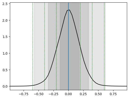
Voilà. You performed a basic parameter inference task with neural ratio estimation. The gray regions should the 68.3%, 95.5% and 99.7% highest density credible regions. The correct regions are indicated by the green vertical lines. The result will not be perfect, but we will discuss later possible ways to improve.

Exercises

1. The swyft.Samples object is compatible with array slicing operatios (details). Extract the first 3 samples from the samples object by using numpy array slicing notation.

# Your results goes here

2. The return type of swyft.LogRatioEstimator_1dim, and in the above example of the inference network, is swyft.LogRatioSamples.

• Confirm that this is also the type of the predictions returned by the infer method.

• Extract \(\ln r(x; z)\) (contained in the logratios variable) as well as the parameter \(z\) (contained in the params variable) from the predictions.

• Plot \(\ln r(x;z)\) vs \(z\) using plt.scatter (make sure to pass everything as vectors).

# Your results goes here

This page was generated from notebooks/0A - SwyftModule.ipynb.